4.2 Using the Descriptive Statistics in Excel to Obtain the Measures

Sample 1

1. Go to Data > Data Analysis.
2. Select Descriptive Statistics and click OK.

Note: If Data Analysis does not appear in the Data menu, refer to the instructions in Lab 1 Getting Started with Excel how to make it available.

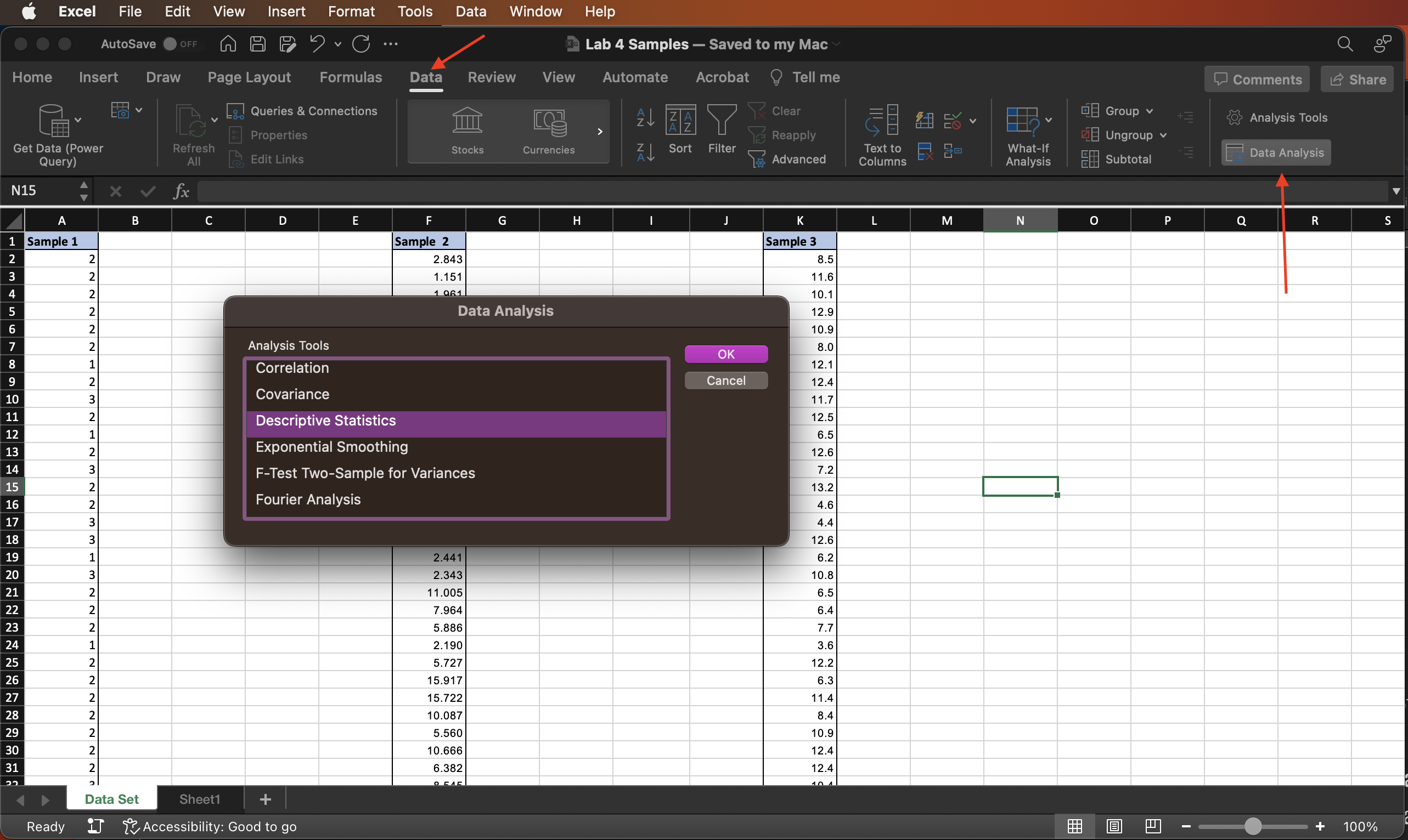
Figure 4.1: Data Analysis dialog window.

3. The Descriptive Statistics window should appear. Complete the Descriptive Statistics window with the information needed from the data in Sample 1.
4. The Input Range for Sample 1 has cell address $A$2:$A$101 (not including the label). If you include the label cell in the address, the address is $A$1:$A$101 (the first cell address is different). You may want to fill in the input range by manually typing the address or by selecting the cells.
5. If the data values are stacked in a column, then check the options Grouped by Columns. If they were entered into Rows instead, then you would select the rows option.
6. After you filled in the input range field, check or uncheck the box Labels in the first row according to what is in the input range.
7. Check the option Output Range and select a cell in a blank area of your worksheet. 8.Check the option Summary statistics.
8. Click OK.

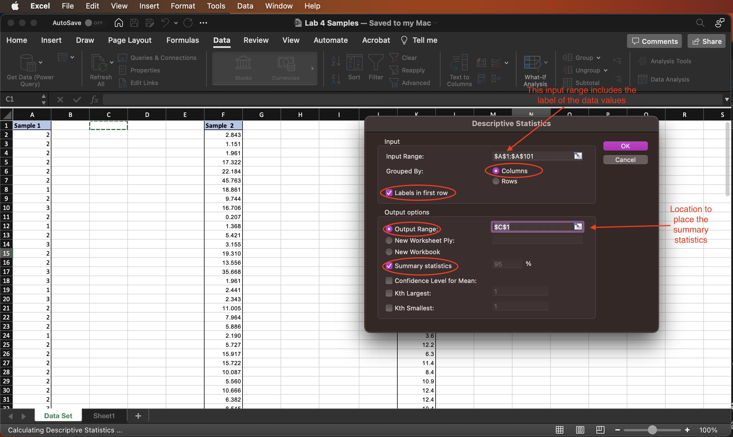
Figure 4.2: Descriptive Statistics dialog window.

These options give you the statistics of Sample 1 such as mean, median, standard deviation, and others.

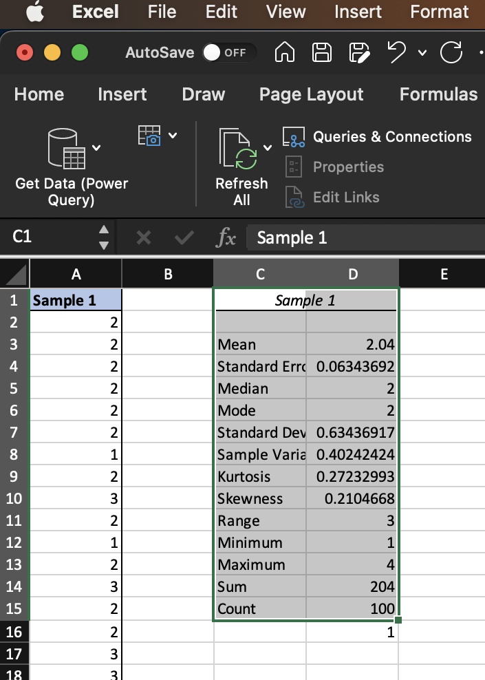
Figure 4.3: The resulting summary statistics for Sample 1.

4.2.1 Practice 1

Now you will do the same work above (Steps 1-8) for Samples 2 and 3.

Note: In the instructions above, you must adjust the cell addresses for Samples 2 and 3.