7.3 Percentile Ranks
The function PERCENTRANK.INC(array, x, [significance]) calculates a specific value’s relative position within a data set, expressed as a percentile rank between 0 and 1, inclusive. Significance is an optional argument. that identifies the number of significant digits for the returned percentage value. If omitted, PERCENTRANK.INC uses three digits (0.xxx).
Example: Suppose that a data set contains the test scores for a class of 20 students, and you want to find the percentile rank of the value in cell A1. You would use the following formula =PERCENTRANK.INC(A1). This formula will return the corresponding percentile of the value with three (3) decimal places.
- Go to the top of another empty column and type Hawaii Measure as the header of the column.
- Copy the values in cells C4:C21 and paste them below the header Hawaii Measure.
- Below Percentile Rank, enter the formula
=PERCENTRANK.INC ($O$2:$O$19,O2). - Select the cell containing the formula above.
- Position the mouse pointer in the lower right corner of the selected cell until it becomes a
+sign and click-drag downward across the range that covers all the values in Step 3. The results are in the decimal form.
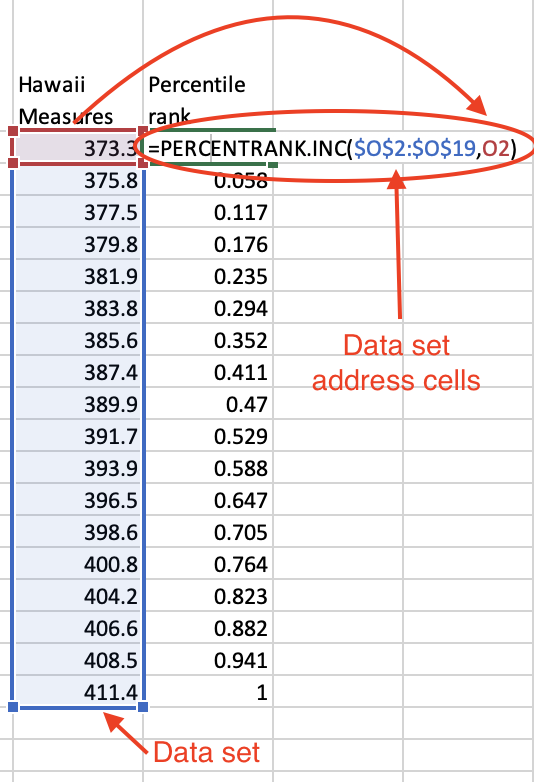
Figure 7.2: Percentile rank calculations for the Hawaii measures.
Note: To convert the results to percentages, select the values in the column Percentile Rank, go to the Home tab, and then change the format to Percentages in the Number ribbon.
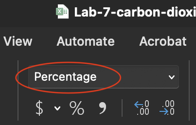
Figure 7.3: Numbers ribbon in the Home tab displaying the Percentage format.