1.6 The Excel Workbook
The workbook is an Excel file that consists of one or more worksheets. The tabs near the bottom of the screen show that we are working with Sheet 1 (check Figures 1.1 and 1.2) . To change worksheets, click on the corresponding worksheet tab. Alternatively, you can RIGHT-click (or Control + click) the arrows just to the left of the worksheet tabs to get a list of all the worksheets in the projects and select a worksheet.
1.6.1 The Cells in the Worksheet
When you look at a worksheet, you should see horizontal and vertical grid lines. Grid lines are light grey lines that appear around cells on Microsoft Excel worksheets. If they are missing, you will need to activate that feature. To do so, see lines:
- Select the
Viewtab. - Click the
Showgroup on the tab. - Be sure that the
Gridlinesoption is checked or selected.
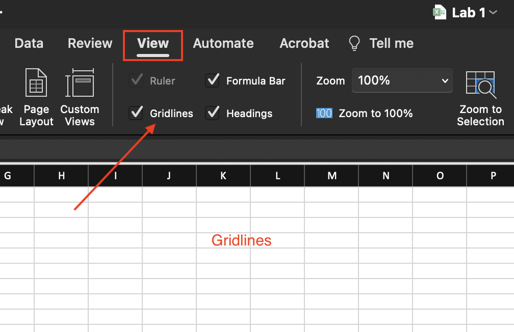
Figure 1.16: Gridlines option in the View tab.
1.6.2 Cell Addresses
Intersecting rows and columns form the cells. A cell’s address consists of a column letter followed by a row number. For example, address B3 designates the cell in Column B, Row 3. When Cell B3 is highlighted, it is the active cell, which means we can enter text or numbers into Cell B3.
1.6.3 Selecting Cells
To select a cell, position the cursor in the cell and click the left mouse button (or click on your computer’s trackpad). Sometimes you will want to select several cells simultaneously to format them (as described next).
To select a rectangular block of cells, position the cursor in a corner cell, hold down the left mouse button, drag the cursor to the cell in the opposite corner of the block, and release the button.
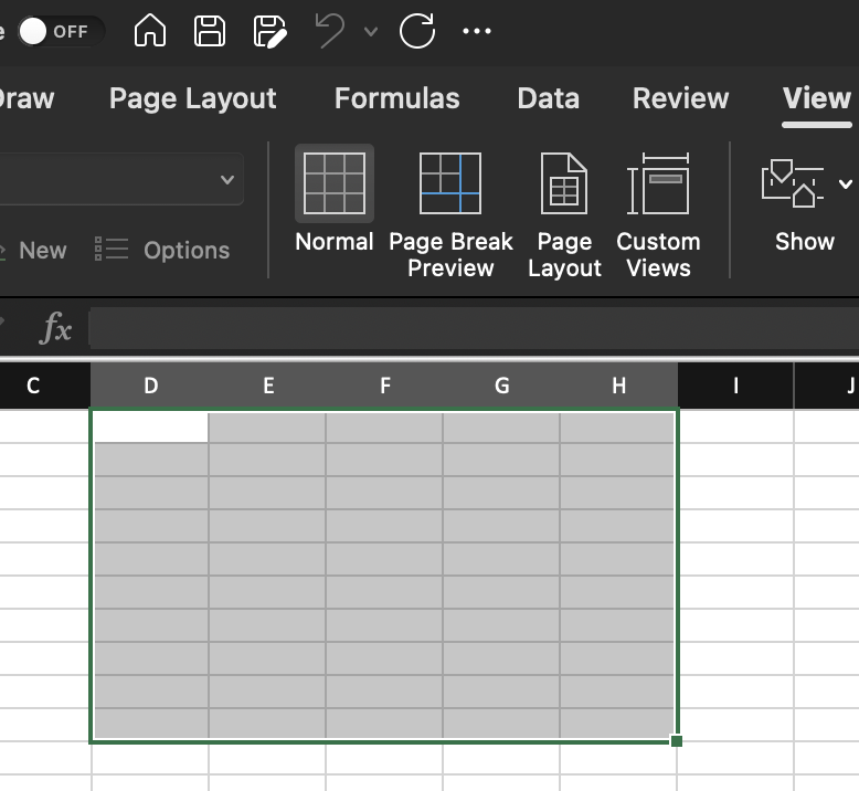
Figure 1.17: A block of cells selected in the worksheet.
To select an entire column, click on the letter above the column to be selected; to select an entire row, click on the number to its left.
To select every cell in the worksheet, click on the blank gray rectangle in the upper left corner of the worksheet (above row header 1 and left of column header A).
You can also select a block of cells by typing the two corner cells into the active cell address window. For example, typing B3:E4 and pressing Enter would select the rectangular block of cells from B3 to the opposite corner E4.
1.6.4 Formatting Cell Contents
In Excel, you may place text or numbers in a cell. As in other Windows applications, you can format the text or numbers by using the formatting toolbar buttons for bold (B), italics (I), underline (U), etc. Other options include left, right, and centered alignment within a cell.
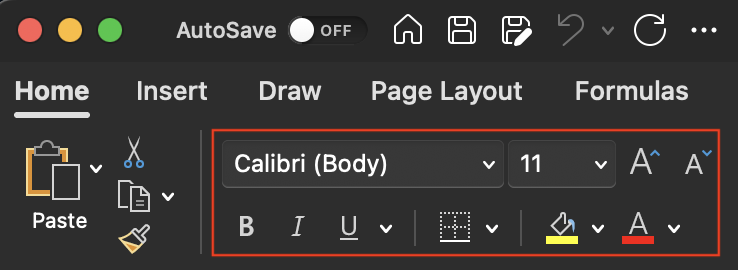
Figure 1.18: Text Formatting ribbon in the Home tab.
Numbers can be formatted to represent dollar amounts ($) or percent form (%) and can be shown with commas in large numbers (,). The number of decimal places to which numbers are carried is also adjustable. All these options appear on the formatting menu bar. Other options are accessible by RIGHT-clicking on a cell and selecting Format Cells.
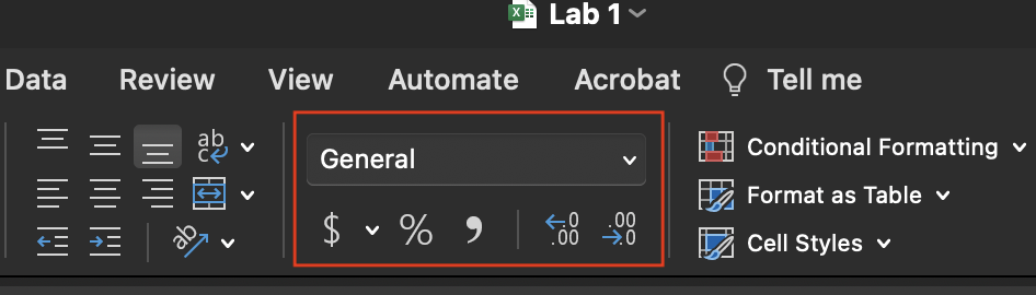
Figure 1.19: Number Formatting ribbon in the Home tab.
1.6.5 Changing Cell Width
Column widths and row heights can be adjusted by placing the cursor between two columns’ letters or row numbers. Hold the left mouse button down when the cursor changes appearance, move the column or row boundary, and release. All these instructions may seem a little mysterious, but once you try them, you will find that they are fairly easy to remember.